The RBF-SVM Visualizer: Watching the Kernel Trick Think

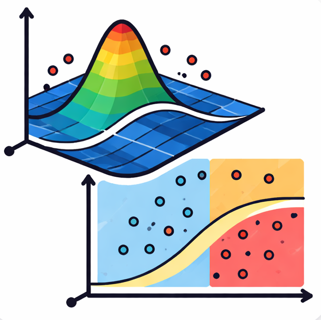
A straight line rarely divides the world. Most interesting boundaries — a tumor from healthy tissue, spam from ham, one speaker's voice from another — are curved, nested, entangled. The support vector machine's answer is not to draw a better line, but to lift the data into a space where a line *will* do, and then draw it there. This project is a from-scratch simulator that makes that lift visible.

The classical SVM finds the maximum-margin hyperplane that separates two classes. But the moment real data stops being linearly separable, that hyperplane stops existing. The RBF-SVM Visualizer demonstrates the standard escape hatch — the kernel trick — by computing the decision function over an entire grid and rendering both the flat 2D classification regions and the 3D “topography” of the decision score. You can watch a non-linear boundary assemble itself as you tune $\gamma$ and $C$.¹

The problem: linear separability

In its simplest form, a support vector machine seeks the maximum-margin hyperplane dividing two classes. Most real datasets, however, are not linearly separable in their original feature space. Forcing a linear boundary produces high misclassification and poor generalization.

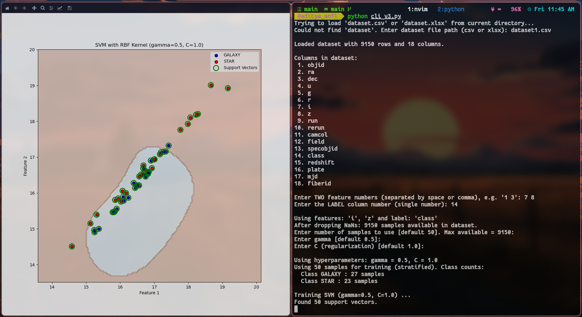Figure 1 — The CLI plots the raw point cloud, then projects it into the 3D decision-score space where the kernel’s separation becomes apparent.

The kernel trick resolves this without ever materializing the high-dimensional mapping. Instead of transforming features and then computing a dot product, we use a kernel function $K(x,x^{\prime })$ that returns the dot product as if the points had been transformed — at a fraction of the cost.²

The Radial Basis Function kernel

The RBF kernel — also called the Gaussian kernel — is the default choice for non-linear SVMs. It is defined as:

$$K(x,x^{\prime })=\exp (-\gamma \Vert x-x^{\prime }{\Vert }^2)$$

Here $\Vert x-x^{\prime }{\Vert }^2$ is the squared Euclidean distance, and $\gamma$ (gamma) controls the radius of influence of a single training point.

• High $\gamma$ → a tighter, more localized influence; the model fits the training data closely and risks overfitting.
• Low $\gamma$ → a broader, smoother boundary; the model underfits but generalizes.

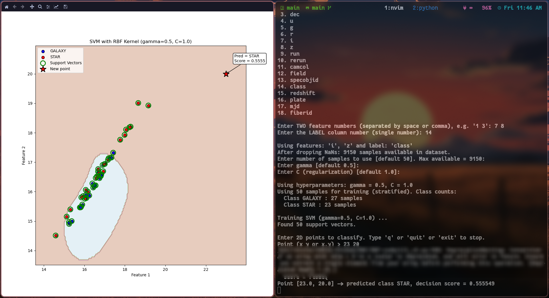Figure 2 — Dropping a custom query point updates both the 2D contour and the 3D surface in real time, showing which side of the margin it lands on.

From the dual problem to the decision surface

The visualizer builds the decision boundary by solving the SVM’s dual optimization problem with Quadratic Programming. The objective is:

$$\underset{\alpha }{\min }\frac{1}{2}\sum _{i,j=1}^n{\alpha }_i{\alpha }_j{y}_i{y}_{j}K(x_i,x_j)-\sum _{i=1}^n{\alpha }_i$$

subject to $0\le {\alpha }_i\le C$ and ${\sum }_i{\alpha }_i{y}_i=0$, where $C$ is the regularization parameter. Points with ${\alpha }_i>0$ become the support vectors — the only points that actually define the boundary.

Once the optimal $\alpha$ values are found, the decision function for any new point $x$ is:

$$f(x)=\sum _{i\in SV}{\alpha }_i{y}_{i}K(x_i,x)+b$$

The renderer maps $f(x)$ across a grid. In 2D this appears as shaded class regions; in 3D the decision score becomes the $Z$-axis, producing a topographical map of classification confidence.

System architecture

The simulator is organized as four cooperating stages:

1. Input module — loads CSV or XLSX datasets and lets you pick which columns are features vs. labels.
2. Computational engine — implements the Gaussian RBF kernel and drives the QP solver (CVXOPT) to recover the Lagrange multipliers $\alpha$.
3. Inference engine — evaluates $f(x)$ for new points and classifies them using the support vectors.
4. Rendering module — Matplotlib produces static 2D contours and an interactive 3D decision surface.

Using the simulator

The CLI gives a scriptable workflow for plotting data and running live predictions; the GUI adds a Tkinter dashboard for dragging $\gamma$ and $C$ and watching the surface deform.

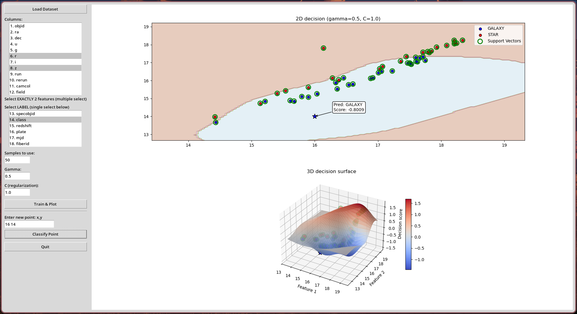Figure 3 — The GUI exposes hyperparameter sliders and support-vector highlighting for exploratory teaching.

A minimal session looks like:

from rbf_svm import RBFSVM
 
model = RBFSVM(gamma=0.5, C=1.0)
model.fit(X_train, y_train)
 
# decision score at every grid point -> 2D/3D surface
Z = model.decision_surface(X_grid)
y_pred = model.predict(X_test)

Interactive features worth calling out:

• Hyperparameter adjustment — live modification of $\gamma$ and $C$.
• Live classification — type arbitrary coordinates, get an immediate prediction.
• Support-vector highlighting — points on the margin are visually distinguished.

Why visualization matters

Mathematical abstractions are hard to intuit. Showing the 2D and 3D views side by side makes three things concrete:

• The 0-level set — exactly where the surface crosses the feature plane is the decision boundary.
• Margin geometry — how $C$ lets some points be “ignored” to keep the boundary smooth.
• Hyperparameter sensitivity — the immediate visual consequence of changing $\gamma$ on the peaks and valleys of the surface.

Key challenges

• Scalability — the kernel matrix is $N\times N$; large datasets get expensive fast.
• Solver conditioning — the QP problem must be well-posed and actually converge.
• UI responsiveness — heavy numerical rendering has to stay fluid in an interactive widget.

Repository

★ rbf-svm-simulator

A from-scratch RBF Support Vector Machine simulator with 2D/3D decision-surface visualization.

0 stars Python No license

View on GitHub →

Further reading

• On the changing work of software engineers — where ML tooling fits into practice.
• The Rasch Model — another case where a clever transformation turns an intractable measurement into a linear one.
• Burges (1998), “A Tutorial on Support Vector Machines for Pattern Recognition” — the canonical introduction.
• The Kernel Trick, explained (distill.pub) — intuitive treatments of high-dimensional mappings.

Footnotes

1. The quadratic program is solved with CVXOPT, a Python package for convex optimization. ↩

2. Formally, a kernel $K$ is a positive semi-definite function; by Mercer’s theorem it corresponds to an inner product in some feature space without computing the mapping explicitly. ↩